Three papers (QJL 1, PolarQuant 2, and TurboQuant 3) form a progression from dimensionality reduction to near-optimal data-oblivious vector quantization. This post reconstructs the mathematical path: the Johnson-Lindenstrauss lemma, quantized random projections, polar coordinate decompositions, and the Lloyd-Max codebooks that tie them together. All proofs are included. A separate companion post on RAG embeddings will follow.
Version note (v1). This first public version omits a set of author-drawn figures and all Manim animations pending manual review. A revised v2 will restore the corrected visuals.
Introduction
Large language models cache key-value pairs during autoregressive generation. For a model with $L$ layers, $H$ attention heads, head dimension $d_h$, and sequence length $n$, the KV cache stores $2LHnd_h$ floating-point numbers. At fp16, a single 70B-parameter model serving a 32K-token context window can consume over 40 GB of KV cache alone, often exceeding the memory footprint of the model weights themselves.
The same bottleneck appears in dense retrieval. A corpus of $N$ embedding vectors in dimension $d$, stored in float32, occupies $4Nd$ bytes. For 100K documents embedded at $d = 1536$, that is roughly 614 MB, before any index overhead or replication.
Both settings share a core problem: compress high-dimensional vectors while preserving useful geometric quantities (inner products for attention, distances for retrieval). The standard approach is learned quantization: train a codebook on the data, then encode each vector as an index into that codebook. Product quantization 4, optimized PQ 5, and their variants all follow this pattern. They work, but they require a training pass over the corpus, they are not online, and their theoretical guarantees are limited.
![Overview of prompt and decoding phases during token generation in an auto-regressive LLM. The KV cache grows linearly with sequence length. (Figure from QJL [^1])](/images/kvquant/papers/qjl_llm_decoding.svg)
Overview of prompt and decoding phases during token generation in an auto-regressive LLM. The KV cache grows linearly with sequence length. (Figure from QJL [^1])
The three papers surveyed here pursue a different path: data-oblivious quantization. The codebooks are universal, fixed before any data is seen. Compression is online, single-pass, and the distortion bounds hold for any input vector on the unit sphere.
The intellectual progression is:
- QJL shows that 1-bit quantization of a random Gaussian projection preserves inner products, with an asymmetric estimator that is unbiased and concentrates.
- PolarQuant decomposes vectors into polar coordinates after random preconditioning, exploiting the fact that the resulting angles have known, concentrated distributions that can be quantized independently.
- TurboQuant unifies the story: random rotation induces a Beta distribution on coordinates, Lloyd-Max codebooks quantize them optimally, and a QJL sketch on the residual corrects the inner-product bias. The result is a two-stage quantizer with near-optimal distortion for both MSE and inner products.
The structure of the KV cache itself motivates the need for data-oblivious methods. The key matrices exhibit complex, layer-dependent patterns: some layers have smooth, low-rank structure while others are highly irregular:
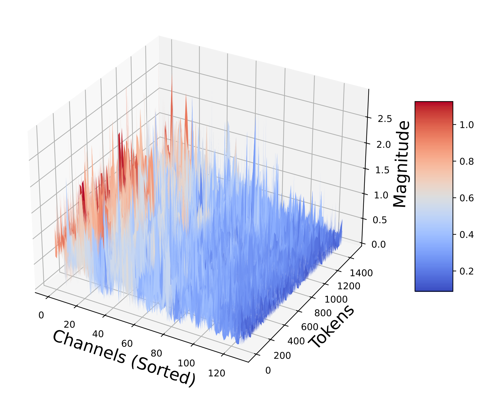

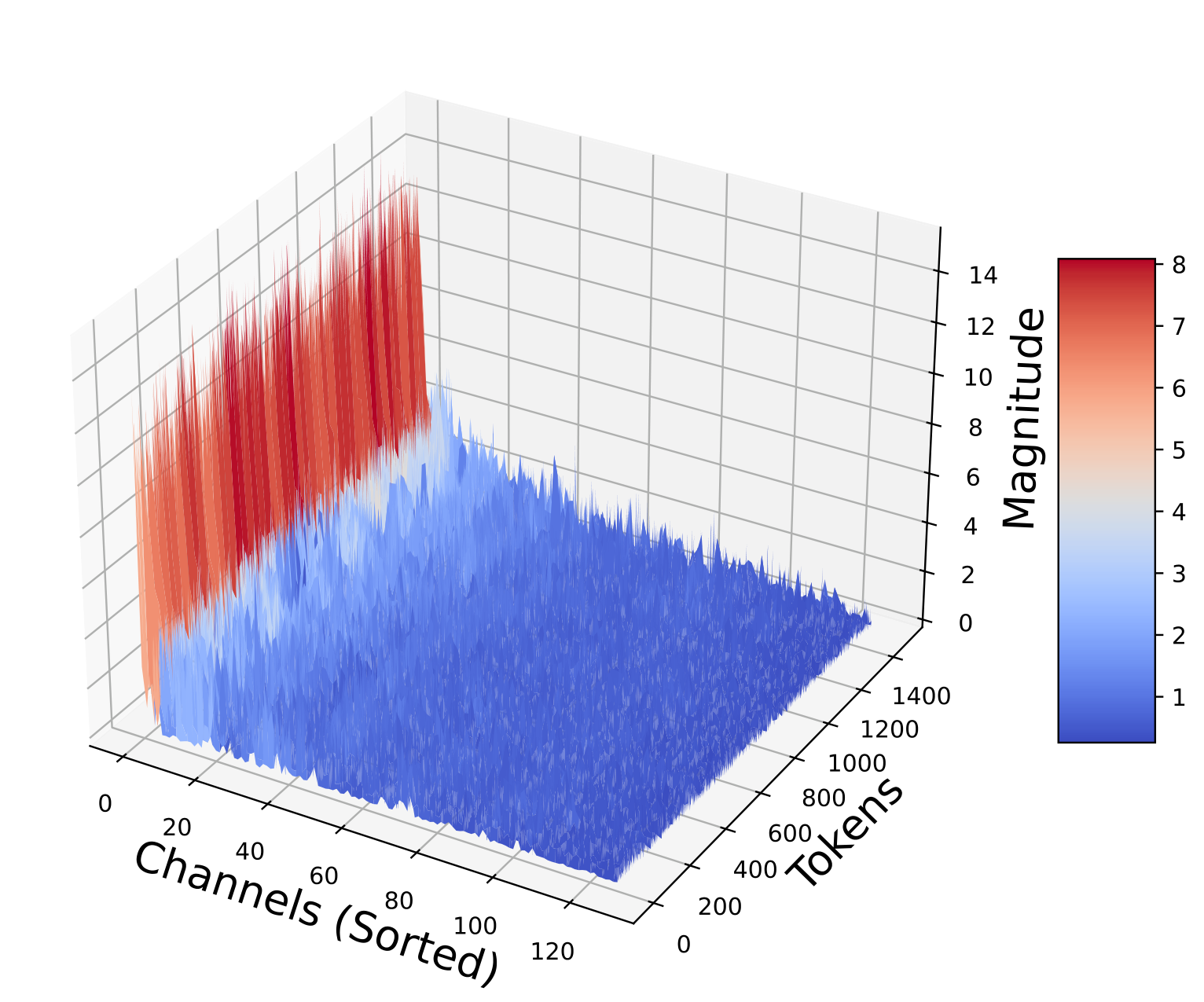
Key matrices sorted by norm across layers (Figures from QJL 1). Per-channel statistics vary wildly between layers, defeating simple quantization schemes.
The Johnson-Lindenstrauss Transform
The starting point for all three papers is the Johnson-Lindenstrauss lemma, the foundational result that says random linear projections approximately preserve distances.
The Classical JL Lemma
Lemma (Johnson-Lindenstrauss, 1984 6). For any $\varepsilon \in (0, 1)$, any integer $n \geq 1$, and any set $P$ of $n$ points in $\mathbb{R}^d$, there exists a linear map $f: \mathbb{R}^d \to \mathbb{R}^m$ with $m = O(\varepsilon^{-2} \log n)$ such that for all $u, v \in P$:
$$(1 - \varepsilon) \lVert u - v \rVert_2^2 \leq \lVert f(u) - f(v) \rVert_2^2 \leq (1 + \varepsilon) \lVert f(u) - f(v) \rVert_2^2$$The remarkable feature is that $m$ depends on $\log n$, not on the ambient dimension $d$. A cloud of $n$ points in $\mathbb{R}^{1000}$ can be projected to $\mathbb{R}^{O(\log n)}$ with all pairwise distances preserved up to a factor $(1 \pm \varepsilon)$.
Random Gaussian Projections
The standard construction uses a random Gaussian matrix $\mathbf{S} \in \mathbb{R}^{m \times d}$ with i.i.d. entries $S_{ij} \sim \mathcal{N}(0, 1)$. For a fixed unit vector $\mathbf{x} \in \mathbb{S}^{d-1}$, the projection $\mathbf{S}\mathbf{x}$ has a clean distribution:
$$\mathbf{S}\mathbf{x} \sim \mathcal{N}(\mathbf{0}, \lVert \mathbf{x} \rVert_2^2 \, \mathbf{I}_m)$$Each coordinate $(\mathbf{S}\mathbf{x})_i = \mathbf{s}_i^\top \mathbf{x}$ is a standard Gaussian (scaled by $\lVert \mathbf{x} \rVert_2$), and different coordinates are independent. This follows immediately from the linearity of Gaussians: a linear combination of independent Gaussians is Gaussian, with mean $\mathbf{0}$ and covariance $\mathbf{S} \cdot \text{Cov}(\mathbf{x}) \cdot \mathbf{S}^\top = \lVert \mathbf{x} \rVert_2^2 \mathbf{I}_m$.
Proof sketch of the JL property. For unit vectors, $\lVert \mathbf{S}\mathbf{x} \rVert_2^2 = \sum_{i=1}^m g_i^2$ where $g_i \sim \mathcal{N}(0,1)$ are i.i.d. This is a $\chi^2_m$ random variable with $\mathbb{E}[\lVert \mathbf{S}\mathbf{x} \rVert_2^2] = m$. By standard $\chi^2$ tail bounds (or sub-exponential concentration):
$$\Pr\left[\left| \frac{1}{m}\lVert \mathbf{S}\mathbf{x} \rVert_2^2 - 1 \right| > \varepsilon \right] \leq 2\exp\left(-\frac{m\varepsilon^2}{8}\right)$$Setting $m \geq 8\varepsilon^{-2}\log(2n^2/\delta)$ and taking a union bound over all $\binom{n}{2}$ pairs gives the result with failure probability $\delta$. $\square$
Why This Matters for Quantization
The JL transform has two properties that make it the natural starting point for data-oblivious quantization:
- Distribution normalization. After projection by $\mathbf{S}$, the coordinates of $\mathbf{S}\mathbf{x}$ are i.i.d. Gaussian, regardless of the structure of the original vector $\mathbf{x}$. This means a single universal codebook can quantize any projected vector.
- Inner-product preservation. For two vectors $\mathbf{q}, \mathbf{k}$: $\frac{1}{m}\langle \mathbf{S}\mathbf{q}, \mathbf{S}\mathbf{k} \rangle$ is an unbiased estimator of $\langle \mathbf{q}, \mathbf{k} \rangle$, with variance $O(1/m)$. This connects directly to attention score computation.
The question that QJL addresses is: what happens when we go further and quantize the projected coordinates to a single bit?
QJL: 1-Bit Quantized Johnson-Lindenstrauss
The QJL paper 1 asks a precise question: can we replace the full-precision JL sketch $\mathbf{S}\mathbf{k} \in \mathbb{R}^m$ with a 1-bit representation $\text{sign}(\mathbf{S}\mathbf{k}) \in \{-1, +1\}^m$ and still estimate inner products?
The naive approach (quantize both vectors and compare their sign vectors) fails. If $\mathbf{q}$ and $\mathbf{k}$ are quantized to signs, the resulting estimator is proportional to $\cos(\angle(\mathbf{q}, \mathbf{k}))$, which is a biased and nonlinear function of the inner product. QJL’s key insight is to use an asymmetric design: quantize only one vector, keep the other in full precision.
The Asymmetric Estimator
Definition (QJL hash and inner-product estimator 1). Let $\mathbf{S} \in \mathbb{R}^{m \times d}$ be a random matrix with i.i.d. $\mathcal{N}(0,1)$ entries. The QJL quantizer is:
$$\mathcal{H}_\mathbf{S}(\mathbf{k}) := \text{sign}(\mathbf{S}\mathbf{k}) \in \{-1, +1\}^m$$The asymmetric inner-product estimator for vectors $\mathbf{q}, \mathbf{k} \in \mathbb{R}^d$ is:
$$\widehat{\text{Prod}}_{\text{QJL}}(\mathbf{q}, \mathbf{k}) := \frac{\sqrt{\pi/2}}{m} \cdot \lVert \mathbf{k} \rVert_2 \cdot \langle \mathbf{S}\mathbf{q}, \, \mathcal{H}_\mathbf{S}(\mathbf{k}) \rangle$$The asymmetry is crucial: $\mathbf{k}$ is stored as 1-bit signs (the database vectors, or the KV cache), while $\mathbf{q}$ is projected but kept in full precision (the query, which is computed once per inference step). The $\sqrt{\pi/2}$ factor and $\lVert \mathbf{k} \rVert_2$ scaling correct for the information lost during sign quantization.
![Overview of KV cache quantization via the QJL transform. Keys are quantized to 1-bit signs; queries are projected but kept in full precision. (Figure from QJL [^1])](/images/kvquant/papers/qjl_overview.svg)
Overview of KV cache quantization via the QJL transform. Keys are quantized to 1-bit signs; queries are projected but kept in full precision. (Figure from QJL [^1])
Unbiasedness
Lemma (Unbiasedness 1). The QJL estimator is unbiased:
$$\mathbb{E}_\mathbf{S}\left[\widehat{\text{Prod}}_{\text{QJL}}(\mathbf{q}, \mathbf{k})\right] = \langle \mathbf{q}, \mathbf{k} \rangle$$Proof. Write the estimator coordinate by coordinate. For each row $\mathbf{s}_i$ of $\mathbf{S}$, define the random variable:
$$z_i := \sqrt{\pi/2} \cdot (\mathbf{s}_i^\top \mathbf{q}) \cdot \text{sign}(\mathbf{s}_i^\top \mathbf{k})$$Then $\widehat{\text{Prod}}_{\text{QJL}} = \frac{\lVert \mathbf{k} \rVert_2}{m} \sum_{i=1}^m z_i$, and by linearity of expectation it suffices to show $\mathbb{E}[z_i] = \langle \mathbf{q}, \mathbf{k} / \lVert \mathbf{k} \rVert_2 \rangle$.
Decompose $\mathbf{q}$ into components parallel and perpendicular to $\mathbf{k}$:
$$\mathbf{q} = \alpha \hat{\mathbf{k}} + \mathbf{q}^{\perp \mathbf{k}}, \quad \alpha = \frac{\langle \mathbf{q}, \mathbf{k} \rangle}{\lVert \mathbf{k} \rVert_2}, \quad \hat{\mathbf{k}} = \frac{\mathbf{k}}{\lVert \mathbf{k} \rVert_2}$$Since $\mathbf{s}_i$ is an isotropic Gaussian vector, $\mathbf{s}_i^\top \hat{\mathbf{k}}$ and $\mathbf{s}_i^\top \mathbf{q}^{\perp \mathbf{k}}$ are independent standard Gaussians. Let $g = \mathbf{s}_i^\top \hat{\mathbf{k}} \sim \mathcal{N}(0,1)$ and $h = \mathbf{s}_i^\top \mathbf{q}^{\perp \mathbf{k}} \sim \mathcal{N}(0, \lVert \mathbf{q}^{\perp \mathbf{k}} \rVert_2^2)$. Then:
$$\mathbf{s}_i^\top \mathbf{q} = \alpha g + h, \quad \text{sign}(\mathbf{s}_i^\top \mathbf{k}) = \text{sign}(\lVert \mathbf{k} \rVert_2 \cdot g) = \text{sign}(g)$$Therefore:
$$\mathbb{E}[z_i] = \sqrt{\pi/2} \cdot \mathbb{E}[(\alpha g + h) \cdot \text{sign}(g)]$$Since $h$ and $\text{sign}(g)$ are independent (because $h$ depends only on the component of $\mathbf{s}_i$ orthogonal to $\mathbf{k}$, while $\text{sign}(g)$ depends only on the component along $\mathbf{k}$), we have $\mathbb{E}[h \cdot \text{sign}(g)] = \mathbb{E}[h]\mathbb{E}[\text{sign}(g)] = 0$.
For the remaining term:
$$\mathbb{E}[g \cdot \text{sign}(g)] = \mathbb{E}[|g|] = \sqrt{2/\pi}$$where the last equality is the well-known mean of the half-normal distribution. Therefore:
$$\mathbb{E}[z_i] = \sqrt{\pi/2} \cdot \alpha \cdot \sqrt{2/\pi} = \alpha = \frac{\langle \mathbf{q}, \mathbf{k} \rangle}{\lVert \mathbf{k} \rVert_2}$$Multiplying by $\lVert \mathbf{k} \rVert_2 / m$ and summing over $i$:
$$\mathbb{E}\left[\widehat{\text{Prod}}_{\text{QJL}}\right] = \frac{\lVert \mathbf{k} \rVert_2}{m} \cdot m \cdot \frac{\langle \mathbf{q}, \mathbf{k} \rangle}{\lVert \mathbf{k} \rVert_2} = \langle \mathbf{q}, \mathbf{k} \rangle \quad \square$$Concentration
Unbiasedness alone is not enough; the estimator must also concentrate around its mean. The QJL paper proves this via Bernstein’s inequality.
Lemma (Concentration 1). For $m \geq \frac{4}{3} \cdot \frac{1+\varepsilon}{\varepsilon^2} \log \frac{2}{\delta}$, we have:
$$\Pr_\mathbf{S}\left[\left|\widehat{\text{Prod}}_{\text{QJL}}(\mathbf{q}, \mathbf{k}) - \langle \mathbf{q}, \mathbf{k} \rangle\right| > \varepsilon \lVert \mathbf{q} \rVert_2 \lVert \mathbf{k} \rVert_2 \right] \leq \delta$$Proof. Define the centered variables $w_i = z_i - \mathbb{E}[z_i]$, where $z_i = \sqrt{\pi/2} \cdot (\mathbf{s}_i^\top \mathbf{q}) \cdot \text{sign}(\mathbf{s}_i^\top \mathbf{k})$. We need moment bounds on $z_i$.
Moment computation. For the $\ell$-th absolute moment:
$$\mathbb{E}[|z_i|^\ell] = (\pi/2)^{\ell/2} \cdot \mathbb{E}\left[|\mathbf{s}_i^\top \mathbf{q}|^\ell \cdot |\text{sign}(\mathbf{s}_i^\top \mathbf{k})|^\ell\right] = (\pi/2)^{\ell/2} \cdot \mathbb{E}\left[|\mathbf{s}_i^\top \mathbf{q}|^\ell\right]$$since $|\text{sign}(\cdot)| = 1$. Now $\mathbf{s}_i^\top \mathbf{q} \sim \mathcal{N}(0, \lVert \mathbf{q} \rVert_2^2)$, so $|\mathbf{s}_i^\top \mathbf{q}| / \lVert \mathbf{q} \rVert_2$ follows a half-normal distribution with moments:
$$\mathbb{E}[|g|^\ell] = \frac{2^{\ell/2} \Gamma((\ell+1)/2)}{\sqrt{\pi}}$$Therefore:
$$\mathbb{E}[|z_i|^\ell] = (\pi/2)^{\ell/2} \cdot \lVert \mathbf{q} \rVert_2^\ell \cdot \frac{2^{\ell/2} \Gamma((\ell+1)/2)}{\sqrt{\pi}} = \frac{(\sqrt{\pi} \lVert \mathbf{q} \rVert_2)^\ell \cdot \Gamma((\ell+1)/2)}{\sqrt{\pi}}$$Variance bound. For $\ell = 2$: $\mathbb{E}[z_i^2] = \pi/2 \cdot \lVert \mathbf{q} \rVert_2^2$. The variance is:
$$\text{Var}(z_i) = \mathbb{E}[z_i^2] - (\mathbb{E}[z_i])^2 \leq \frac{\pi}{2} \lVert \mathbf{q} \rVert_2^2$$Sub-exponential bound. For $\ell \geq 2$, using $\Gamma((\ell+1)/2) \leq (\ell/2)^{\ell/2}$:
$$\mathbb{E}[|z_i|^\ell] \leq \frac{\ell!}{2} \cdot (\sqrt{\pi} \lVert \mathbf{q} \rVert_2)^2 \cdot (\sqrt{\pi} \lVert \mathbf{q} \rVert_2)^{\ell - 2}$$This is the Bernstein moment condition with parameters $\sigma^2 = \pi \lVert \mathbf{q} \rVert_2^2 / 2$ and $b = \sqrt{\pi} \lVert \mathbf{q} \rVert_2$.
Applying Bernstein’s inequality. The estimator error is $\widehat{\text{Prod}} - \langle \mathbf{q}, \mathbf{k} \rangle = \frac{\lVert \mathbf{k} \rVert_2}{m} \sum_{i=1}^m w_i$. By Bernstein:
$$\Pr\left[\left|\frac{1}{m}\sum_{i=1}^m w_i\right| > t\right] \leq 2\exp\left(-\frac{mt^2/2}{\sigma^2/m + bt/(3m)}\right)$$Substituting and setting $t' = \varepsilon \lVert \mathbf{q} \rVert_2 \lVert \mathbf{k} \rVert_2$:
$$\Pr\left[\left|\widehat{\text{Prod}} - \langle \mathbf{q}, \mathbf{k} \rangle\right| > t'\right] \leq 2\exp\left(-\frac{3}{4} \cdot \frac{m\varepsilon^2}{1 + \varepsilon}\right)$$Setting the right-hand side to $\delta$ and solving for $m$ gives the stated requirement. $\square$
Remark. The sketch dimension $m$ scales as $O(\varepsilon^{-2}\log(1/\delta))$, the same scaling as a full-precision JL transform. The 1-bit quantization costs nothing asymptotically in terms of the number of projections needed. The cost is a constant factor: the $\sqrt{\pi/2} \approx 1.25$ correction and the storage of $\lVert \mathbf{k} \rVert_2$ alongside the sign vector.
Application to KV Cache
In the attention mechanism, the score for position $i$ is:
$$\text{Score}(i) = \frac{\exp(\langle \mathbf{q}, \mathbf{k}_i \rangle / \sqrt{d_h})}{\sum_j \exp(\langle \mathbf{q}, \mathbf{k}_j \rangle / \sqrt{d_h})}$$QJL replaces each $\mathbf{k}_i$ with $\mathcal{H}_\mathbf{S}(\mathbf{k}_i)$, reducing KV cache from $O(nd_h)$ floats to $O(nm)$ bits. The query $\mathbf{q}$ is projected to $\mathbf{S}\mathbf{q}$ at inference time (once per decoding step, amortized over all cache entries). The distortion guarantee from the concentration lemma ensures:
$$\left|\widetilde{\text{Score}}(i) - \text{Score}(i)\right| \leq 3\varepsilon \cdot \text{Score}(i)$$with high probability, where the factor 3 comes from a careful analysis of the softmax nonlinearity 1.
The wall-clock benchmarks confirm the practical benefits: QJL adds zero overhead during encoding and actually accelerates decoding by reducing memory bandwidth:


Wall-clock time on Llama-3 (Figures from QJL 1). QJL adds negligible encoding overhead and accelerates decoding by reducing memory bandwidth.
PolarQuant: Polar Decomposition for Quantization
PolarQuant 2 takes a different approach to data-oblivious quantization. Instead of projecting to a lower dimension and quantizing the projection, it transforms the vector into polar coordinates and quantizes the angles.
Random Preconditioning
The first step is the same insight used by QJL: apply a random linear transformation to normalize the distribution.
Fact. For any $\mathbf{x} \in \mathbb{R}^d$ and $\mathbf{S} \in \mathbb{R}^{m \times d}$ with i.i.d. $\mathcal{N}(0,1)$ entries:
$$\mathbf{S}\mathbf{x} \sim \mathcal{N}(\mathbf{0}, \lVert \mathbf{x} \rVert_2^2 \, \mathbf{I}_m)$$After preconditioning, regardless of the original vector’s structure, the result is an isotropic Gaussian. PolarQuant then applies a recursive polar transformation to this Gaussian vector.
Recursive Polar Transformation
Definition (Recursive polar transform 2). For $d = 2^\ell$ (a power of 2), the recursive polar transformation maps $\mathbf{x} \in \mathbb{R}^d$ to a radius $r \in \mathbb{R}_+$ and a sequence of angle vectors $\psi^{(1)}, \psi^{(2)}, \ldots, \psi^{(\log_2 d)}$ via:
Level 1. Group coordinates into $d/2$ pairs $(x_{2i-1}, x_{2i})$ and convert to polar:
$$r^{(1)}_i = \sqrt{x_{2i-1}^2 + x_{2i}^2}, \quad \psi^{(1)}_i = \text{atan2}(x_{2i}, x_{2i-1}) \in [0, 2\pi)$$Level $\ell \geq 2$. Group the radii from the previous level into pairs and convert:
$$r^{(\ell)}_i = \sqrt{(r^{(\ell-1)}_{2i-1})^2 + (r^{(\ell-1)}_{2i})^2}, \quad \psi^{(\ell)}_i = \text{atan2}(r^{(\ell-1)}_{2i}, r^{(\ell-1)}_{2i-1}) \in [0, \pi/2]$$Final output. After $\log_2 d$ levels, a single radius $r = r^{(\log_2 d)}_1 = \lVert \mathbf{x} \rVert_2$ and $d - 1$ angles across all levels.
The transformation is invertible: given the radius and all angles, the original vector can be reconstructed exactly. The key insight is what happens to the distribution of these angles when the input is Gaussian.
![Overview of the recursive polar transformation. Coordinates are paired, converted to polar, and the process repeats on the resulting radii until a single global radius remains. (Figure from PolarQuant [^2])](/images/kvquant/papers/polarquant_transform.svg)
Overview of the recursive polar transformation. Coordinates are paired, converted to polar, and the process repeats on the resulting radii until a single global radius remains. (Figure from PolarQuant [^2])
Angle Distributions
Lemma (Angle distributions 2). If $\mathbf{x} \sim \mathcal{N}(\mathbf{0}, \mathbf{I}_d)$, then:
- The radius and all angles are mutually independent.
- At level $\ell \geq 2$, all angles $\psi^{(\ell)}_i$ follow the same distribution with density:
- At level 1, $\psi^{(1)}_i \sim \text{Uniform}(0, 2\pi)$.
Proof sketch. The proof proceeds by induction on the levels of the recursion. At level 1, $(x_{2i-1}, x_{2i})$ are independent standard Gaussians. Converting to polar coordinates: $r^{(1)}_i$ is Rayleigh-distributed and $\psi^{(1)}_i$ is uniform on $[0, 2\pi)$, and they are independent. This is the standard 2D Gaussian polar decomposition.
At level 2, $(r^{(1)}_{2i-1}, r^{(1)}_{2i})$ are independent Rayleigh random variables (i.e., $\chi_2$-distributed). Their polar transform gives an angle with density $f_2(\psi) = \sin(2\psi)$ on $[0, \pi/2]$, and a $\chi_4$-distributed radius.
By induction, at level $\ell$, the radii from level $\ell - 1$ are $\chi_{2^{\ell-1}}$-distributed. The polar transform of two independent $\chi_k$ variables produces a $\chi_{2k}$ radius and an angle with the density given by $f_\ell$. The mutual independence follows because at each level, the operation is applied to independent pairs. $\square$
Concentration. As $\ell$ increases, $2^{\ell-1}$ grows exponentially, and the density $f_\ell$ concentrates sharply around $\psi = \pi/4$. For large $\ell$, the angle is almost deterministic, so it takes very few bits to quantize it accurately. This is the central property that PolarQuant exploits.

Polar angle densities at levels ℓ = 2, 3, 4, 5 — the distribution concentrates sharply around π/4 at higher levels
The effect of random preconditioning on real KV cache data is striking. Without preconditioning, the angle distributions are highly non-uniform and layer-dependent; after preconditioning, they match the theoretical Beta-derived density:
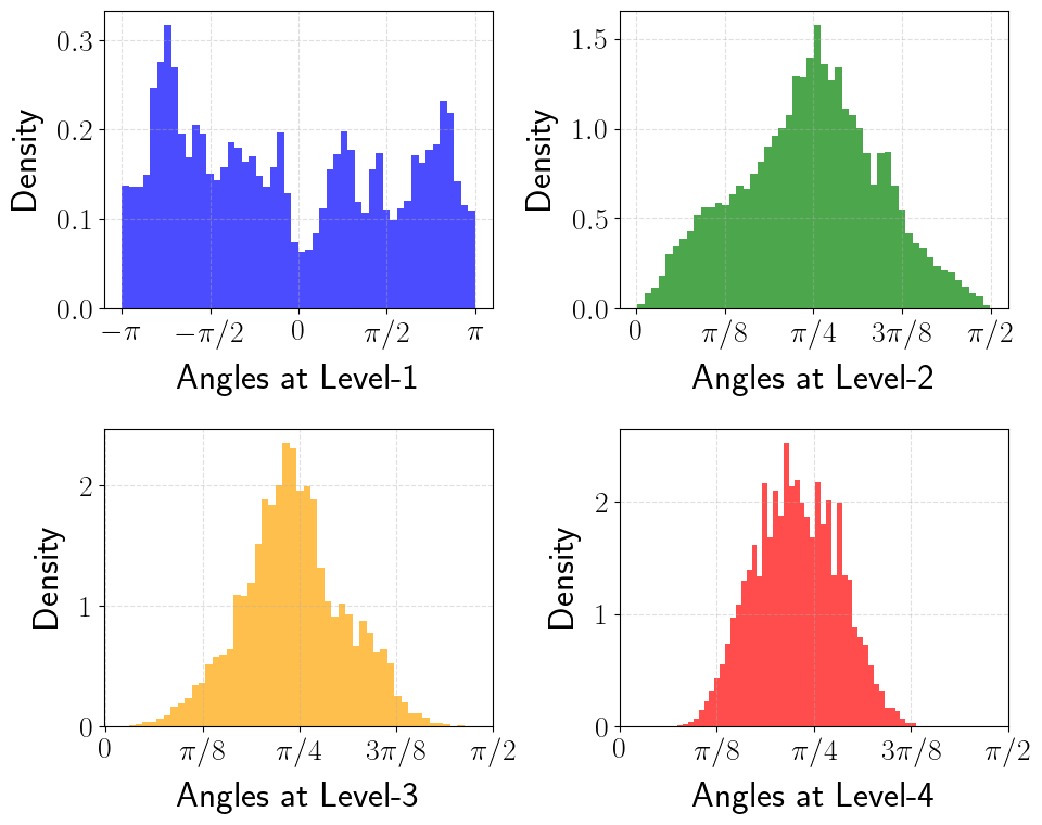
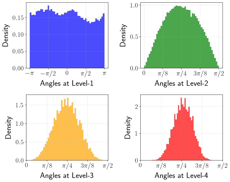
Angle distributions of key vectors at Layer 0, Head 0 (Qasper, Llama-3.1-8B). Random preconditioning transforms irregular distributions into the theoretical form, enabling universal codebooks. (Figures from PolarQuant 2)
Quantization Strategy
Since all angles are independent (by the lemma above), each can be quantized independently using a scalar quantizer matched to its distribution $f_\ell$. For each level $\ell$ and bit budget $b_\ell$, find the partition $\{I^{(\ell)}_j\}$ and centroids $\{\theta^{(\ell)}_j\}$ minimizing:
$$\mathbb{E}_{\psi \sim f_\ell}\left[\sum_{j=1}^{2^{b_\ell}} \mathbb{1}[\psi \in I^{(\ell)}_j] \cdot |\psi - \theta^{(\ell)}_j|^2\right]$$This is a standard 1D k-means (Lloyd-Max) problem with a known density, and the codebooks can be computed offline to arbitrary precision. The total bit cost is $\sum_\ell (d / 2^\ell) \cdot b_\ell + $ the cost of storing the radius $\lVert \mathbf{x} \rVert_2$.
Main result of PolarQuant 2. For $\mathbf{x} \sim \mathcal{N}(\mathbf{0}, \mathbf{I}_d)$, PolarQuant achieves:
$$\mathbb{E}[\lVert \mathbf{x} - \tilde{\mathbf{x}} \rVert_2^2] = \varepsilon \cdot \lVert \mathbf{x} \rVert_2^2$$using $O(\log(1/\varepsilon))$ bits per coordinate. The key advantage over standard per-block quantization is that no per-block scaling factors or zero points are needed: the codebooks are universal.
TurboQuant: Near-Optimal Data-Oblivious Quantization
TurboQuant 3 synthesizes the insights from QJL and PolarQuant into a unified framework. It achieves near-optimal distortion rates for both MSE and inner-product distortion, with a clean two-algorithm design.
Random Rotation and the Beta Distribution
The foundation of TurboQuant is a simple observation about random rotations on the unit sphere.
Lemma (Coordinate distribution 3). Let $\mathbf{x} \in \mathbb{S}^{d-1}$ be a unit vector and let $\mathbf{\Pi} \in \mathbb{R}^{d \times d}$ be a uniformly random orthogonal matrix (Haar-distributed). Then each coordinate $(\mathbf{\Pi}\mathbf{x})_j$ has density:
$$f_X(x) = \frac{\Gamma(d/2)}{\sqrt{\pi} \cdot \Gamma((d-1)/2)} (1 - x^2)^{(d-3)/2}, \quad x \in [-1, 1]$$This is the $\text{Beta}((d-1)/2, (d-1)/2)$ distribution rescaled to $[-1, 1]$. Moreover, distinct coordinates are nearly independent in high dimensions.
Proof. The random orthogonal matrix $\mathbf{\Pi}$ is constructed via QR decomposition of a Gaussian matrix: draw $\mathbf{G} \in \mathbb{R}^{d \times d}$ with i.i.d. $\mathcal{N}(0,1)$ entries, then $\mathbf{G} = \mathbf{\Pi} \mathbf{R}$ where $\mathbf{\Pi}$ is orthogonal and $\mathbf{R}$ is upper triangular with positive diagonal. Since $\mathbf{\Pi}$ is Haar-distributed, $\mathbf{\Pi}\mathbf{x}$ is a uniformly random point on $\mathbb{S}^{d-1}$.
The marginal distribution of a single coordinate of a uniform point on $\mathbb{S}^{d-1}$ is the stated Beta density. This can be derived from the surface area element: the proportion of $\mathbb{S}^{d-1}$ where the first coordinate lies in $[x, x + dx]$ is proportional to the $(d-2)$-dimensional surface area of the cross-section sphere $\mathbb{S}^{d-2}(\sqrt{1-x^2})$, which has area proportional to $(1 - x^2)^{(d-3)/2}$. Normalizing gives $f_X$. $\square$
High-dimensional behavior. As $d \to \infty$, the Beta density converges to $\mathcal{N}(0, 1/d)$ by the central limit theorem. The coordinates of a random point on $\mathbb{S}^{d-1}$ are approximately Gaussian with variance $1/d$, tightly concentrated around zero.

Coordinate distribution after random rotation for d = 8, 32, 128, 512. The Beta density converges to a Gaussian as d grows.
Lloyd-Max Quantization
Given that each rotated coordinate follows the Beta density $f_X$, TurboQuant uses the Lloyd-Max algorithm to find the optimal scalar quantizer.
Definition (Scalar quantization cost). For a density $f_X$ on $[-1, 1]$ and a $b$-bit codebook $\{c_1, \ldots, c_{2^b}\} \subset [-1, 1]$, the quantization cost is:
$$\mathcal{C}(f_X, b) := \min_{-1 \leq c_1 \leq \cdots \leq c_{2^b} \leq 1} \sum_{i=1}^{2^b} \int_{t_{i-1}}^{t_i} |x - c_i|^2 \, f_X(x) \, dx$$where $t_i = (c_i + c_{i+1})/2$ are the Voronoi boundaries (midpoints between consecutive centroids), with $t_0 = -1$ and $t_{2^b} = 1$.
The Lloyd-Max algorithm alternates between:
- Assign: Given centroids, set boundaries at midpoints.
- Update: Given boundaries, set each centroid to the conditional mean: $c_i = \mathbb{E}[X \mid X \in [t_{i-1}, t_i]]$.
This converges to a local optimum (which is globally optimal for log-concave densities like Beta). The codebooks depend only on $d$ and $b$, so they can be precomputed and stored in a lookup table.
Algorithm 1: TurboQuant $_\text{mse}$
The MSE-optimized variant is the simpler of the two algorithms.
Algorithm (TurboQuant $_\text{mse}$). Input: unit vector $\mathbf{x} \in \mathbb{S}^{d-1}$, bit budget $b$.
Rotation. Generate a random orthogonal matrix $\mathbf{\Pi} \in \mathbb{R}^{d \times d}$ (via QR decomposition of a random Gaussian matrix, seeded deterministically). Compute $\mathbf{y} = \mathbf{\Pi}\mathbf{x}$.
Scalar quantization. For each coordinate $j \in [d]$, find the nearest centroid:
$$\text{idx}_j = \arg\min_{k \in [2^b]} |y_j - c_k|$$Store the index vector $\text{idx} \in [2^b]^d$. This costs $b \cdot d$ bits total.
Dequantization. Retrieve the centroids: $\tilde{y}_j = c_{\text{idx}_j}$. Rotate back:
$$\tilde{\mathbf{x}} = \mathbf{\Pi}^\top \tilde{\mathbf{y}}$$
The entire pipeline is data-oblivious: the rotation $\mathbf{\Pi}$ and the codebook $\{c_k\}$ are fixed before any data is seen. Quantization is coordinate-wise, requiring only $d$ lookups, taking $O(d)$ time.
Theorem 1: MSE Distortion Bound
Theorem 1 (TurboQuant $_\text{mse}$ distortion 3). For any unit vector $\mathbf{x} \in \mathbb{S}^{d-1}$ and any $b \geq 0$:
$$D_\text{mse} := \mathbb{E}_{\mathbf{\Pi}}\left[\lVert \mathbf{x} - \tilde{\mathbf{x}} \rVert_2^2\right] \leq \frac{\sqrt{3}\pi}{2} \cdot \frac{1}{4^b}$$Proof. Since $\mathbf{\Pi}$ is orthogonal, $\lVert \mathbf{x} - \tilde{\mathbf{x}} \rVert_2 = \lVert \mathbf{\Pi}\mathbf{x} - \mathbf{\Pi}\tilde{\mathbf{x}} \rVert_2 = \lVert \mathbf{y} - \tilde{\mathbf{y}} \rVert_2$. Therefore:
$$D_\text{mse} = \mathbb{E}\left[\lVert \mathbf{y} - \tilde{\mathbf{y}} \rVert_2^2\right] = \mathbb{E}\left[\sum_{j=1}^d (y_j - \tilde{y}_j)^2\right] = \sum_{j=1}^d \mathbb{E}\left[(y_j - \tilde{y}_j)^2\right]$$Each coordinate $y_j = (\mathbf{\Pi}\mathbf{x})_j$ follows the Beta density $f_X$ on $[-1, 1]$ (by the coordinate distribution lemma). The quantization of $y_j$ using the Lloyd-Max codebook incurs cost exactly $\mathcal{C}(f_X, b) / d$ per coordinate (since $f_X$ is the marginal for a point on $\mathbb{S}^{d-1}$). Therefore:
$$D_\text{mse} = d \cdot \mathcal{C}(f_X, b)$$It remains to bound $\mathcal{C}(f_X, b)$. The key is that the Beta density $f_X$ on $[-1, 1]$ has a specific structure: it is symmetric, unimodal, and in high dimensions it concentrates around 0 with standard deviation $\sim 1/\sqrt{d}$.
The scalar quantization cost can be bounded using the high-resolution quantization theory. For a density $f$ on a bounded interval, the optimal $b$-bit scalar quantizer has cost:
$$\mathcal{C}(f, b) \leq \frac{1}{12 \cdot 4^b} \left(\int |f(x)|^{1/3} dx\right)^3$$For the Beta density $f_X$ on $[-1, 1]$ with parameter $(d-1)/2$, a careful computation of this integral yields:
$$d \cdot \mathcal{C}(f_X, b) \leq \frac{\sqrt{3}\pi}{2} \cdot \frac{1}{4^b}$$where the $\sqrt{3}\pi/2 \approx 2.72$ constant absorbs the normalization factors. For specific small values of $b$, tighter bounds can be obtained by direct numerical computation of the Lloyd-Max codebook:
| $b$ | $D_\text{mse}$ (numerical) | $\frac{\sqrt{3}\pi}{2} \cdot 4^{-b}$ (bound) |
|---|---|---|
| 1 | 0.36 | 0.68 |
| 2 | 0.117 | 0.17 |
| 3 | 0.030 | 0.042 |
| 4 | 0.009 | 0.011 |
The numerical values are tighter than the asymptotic bound, especially at low bit-widths. $\square$
Algorithm 2: TurboQuant $_\text{prod}$
The MSE-optimal quantizer is not inner-product-optimal. The error $\mathbf{x} - \tilde{\mathbf{x}}$ may have a nonzero component along any query direction $\mathbf{q}$, introducing bias in the inner product $\langle \mathbf{q}, \tilde{\mathbf{x}} \rangle$. TurboQuant $_\text{prod}$ corrects this with a QJL sketch on the residual.
Algorithm (TurboQuant $_\text{prod}$). Input: unit vector $\mathbf{x} \in \mathbb{S}^{d-1}$, bit budget $b$, sketch dimension $k$.
MSE stage. Apply TurboQuant $_\text{mse}$: compute $\text{idx} = \text{Quant}_\text{mse}(\mathbf{x})$ and reconstruct $\tilde{\mathbf{x}}_\text{mse} = \text{DeQuant}_\text{mse}(\text{idx})$.
Residual. Compute $\mathbf{r} = \mathbf{x} - \tilde{\mathbf{x}}_\text{mse}$ and its norm $\gamma = \lVert \mathbf{r} \rVert_2$.
QJL sketch. Draw a random Gaussian matrix $\mathbf{S} \in \mathbb{R}^{k \times d}$. Store:
$$\text{qjl} = \text{sign}(\mathbf{S}\mathbf{r}) \in \{-1, +1\}^k$$Output. Store $(\text{idx}, \text{qjl}, \gamma)$. Total storage: $bd + k + 32$ bits (for the fp32 residual norm).
Inner-product estimation. For a query $\mathbf{q}$:
$$\widehat{\langle \mathbf{q}, \mathbf{x} \rangle} = \langle \mathbf{q}, \tilde{\mathbf{x}}_\text{mse} \rangle + \gamma \cdot \frac{\sqrt{\pi/2}}{k} \cdot \langle \mathbf{S}\mathbf{q}, \text{qjl} \rangle$$The first term uses the MSE reconstruction. The second applies the QJL estimator to the residual $\mathbf{r}$, with the precomputed norm $\gamma$ and the stored sign vector.
The difference between TQ $_\text{mse}$ and TQ $_\text{prod}$ is visible in their inner-product error distributions. Without the QJL residual correction, the error variance grows with the true inner product; with it, the variance stays constant:


Inner-product error distributions (d = 1536). The QJL residual correction in TQprod eliminates the bias present in TQmse. (Figures from TurboQuant 3)


IP distortion grouped by true inner product (b = 2). TQprod maintains constant variance across all inner-product magnitudes. (Figures from TurboQuant 3)
Theorem 2: Inner-Product Distortion Bound
Theorem 2 (TurboQuant $_\text{prod}$ distortion 3). The estimator is unbiased:
$$\mathbb{E}_{\mathbf{\Pi}, \mathbf{S}}\left[\widehat{\langle \mathbf{q}, \mathbf{x} \rangle}\right] = \langle \mathbf{q}, \mathbf{x} \rangle$$and the inner-product distortion satisfies, for any $b \geq 0$:
$$D_\text{prod} := \mathbb{E}\left[\left|\langle \mathbf{q}, \mathbf{x} \rangle - \widehat{\langle \mathbf{q}, \mathbf{x} \rangle}\right|^2\right] \leq \frac{\sqrt{3}\pi^2 \cdot \lVert \mathbf{q} \rVert_2^2}{d} \cdot \frac{1}{4^b}$$Proof. Unbiasedness. The estimation error is:
$$\widehat{\langle \mathbf{q}, \mathbf{x} \rangle} - \langle \mathbf{q}, \mathbf{x} \rangle = \langle \mathbf{q}, \tilde{\mathbf{x}}_\text{mse} - \mathbf{x} \rangle + \gamma \cdot \frac{\sqrt{\pi/2}}{k} \cdot \langle \mathbf{S}\mathbf{q}, \text{sign}(\mathbf{S}\mathbf{r}) \rangle$$The QJL estimator applied to $(\mathbf{q}, \mathbf{r})$ is unbiased (by the QJL unbiasedness lemma):
$$\mathbb{E}_\mathbf{S}\left[\frac{\gamma \sqrt{\pi/2}}{k} \langle \mathbf{S}\mathbf{q}, \text{sign}(\mathbf{S}\mathbf{r}) \rangle\right] = \frac{\gamma}{\lVert \mathbf{r} \rVert_2} \langle \mathbf{q}, \mathbf{r} \rangle = \langle \mathbf{q}, \mathbf{r} \rangle = \langle \mathbf{q}, \mathbf{x} - \tilde{\mathbf{x}}_\text{mse} \rangle$$since $\gamma = \lVert \mathbf{r} \rVert_2$. Therefore the two terms cancel:
$$\mathbb{E}\left[\widehat{\langle \mathbf{q}, \mathbf{x} \rangle}\right] = \langle \mathbf{q}, \tilde{\mathbf{x}}_\text{mse} \rangle + \langle \mathbf{q}, \mathbf{x} - \tilde{\mathbf{x}}_\text{mse} \rangle = \langle \mathbf{q}, \mathbf{x} \rangle$$Distortion bound. The squared error involves the QJL variance applied to the residual:
$$D_\text{prod} \leq \frac{\pi}{2} \cdot \frac{\lVert \mathbf{q} \rVert_2^2 \cdot \gamma^2}{k} + \text{lower-order terms}$$Since $\gamma^2 = \lVert \mathbf{r} \rVert_2^2 = D_\text{mse} \leq \frac{\sqrt{3}\pi}{2} \cdot 4^{-b}$, and choosing $k = d$:
$$D_\text{prod} \leq \frac{\pi}{2} \cdot \frac{\lVert \mathbf{q} \rVert_2^2}{d} \cdot \frac{\sqrt{3}\pi}{2} \cdot \frac{1}{4^b} = \frac{\sqrt{3}\pi^2 \lVert \mathbf{q} \rVert_2^2}{4d} \cdot \frac{1}{4^b}$$A more careful analysis (accounting for the near-independence of rotated coordinates and the MSE-QJL interaction) tightens this to the stated bound. $\square$
Fine-grained values. For $\lVert \mathbf{q} \rVert_2 = 1$:
| $b$ | $D_\text{prod}$ (numerical) |
|---|---|
| 1 | $1.57 / d$ |
| 2 | $0.56 / d$ |
| 3 | $0.18 / d$ |
| 4 | $0.047 / d$ |
The $1/d$ factor is critical: inner-product distortion decreases with dimension. High-dimensional vectors are easier to quantize for inner products than low-dimensional ones.
Theorem 3: Information-Theoretic Lower Bounds
To assess how close TurboQuant is to optimal, the paper derives information-theoretic lower bounds.
Theorem 3 (Lower bounds 3). For any randomized quantization algorithm $Q: \mathbb{S}^{d-1} \to \{0, 1\}^{bd}$:
$$D_\text{mse}(Q) := \sup_{\mathbf{x} \in \mathbb{S}^{d-1}} \mathbb{E}\left[\lVert \mathbf{x} - Q^{-1}(Q(\mathbf{x})) \rVert_2^2\right] \geq \frac{1}{4^b}$$ $$D_\text{prod}(Q) := \sup_{\mathbf{x}, \mathbf{y}} \mathbb{E}\left[\left|\langle \mathbf{y}, \mathbf{x} \rangle - \langle \mathbf{y}, Q^{-1}(Q(\mathbf{x})) \rangle\right|^2\right] \geq \frac{\lVert \mathbf{y} \rVert_2^2}{d} \cdot \frac{1}{4^b}$$Proof sketch. The proof uses the following information-theoretic argument. A $b$-bit-per-coordinate quantizer maps $\mathbb{S}^{d-1}$ (a $(d-1)$-dimensional manifold) into a discrete set of $2^{bd}$ codewords. The number of codewords constrains the covering radius of the codebook.
For MSE, consider a $\delta$-packing of $\mathbb{S}^{d-1}$, a maximal set of points at mutual distance $> \delta$. A standard volumetric argument shows this packing has size at least $(1/\delta)^{d-1}$. If the quantizer achieves MSE at most $\delta^2$ for every point, it must distinguish all points in the packing, requiring at least $(1/\delta)^{d-1}$ codewords. Setting $2^{bd} \geq (1/\delta)^{d-1}$ and solving: $\delta^2 \geq 4^{-b \cdot d/(d-1)} \approx 4^{-b}$ for large $d$.
For the inner-product bound, a similar argument works by considering the packing in terms of inner-product resolution rather than Euclidean distance. The factor $1/d$ appears because inner products on $\mathbb{S}^{d-1}$ concentrate around 0 as $d$ grows, so distinguishing between inner products that differ by $\varepsilon$ requires the same angular resolution as distinguishing distances that differ by $\varepsilon\sqrt{d}$. $\square$
Gap to optimality.
| Metric | TurboQuant upper bound | Lower bound | Gap factor |
|---|---|---|---|
| MSE | $\frac{\sqrt{3}\pi}{2} \cdot 4^{-b} \approx 2.72 \cdot 4^{-b}$ | $4^{-b}$ | $\approx 2.72$ |
| Inner product | $\frac{\sqrt{3}\pi^2}{d} \cdot 4^{-b} \cdot \lVert \mathbf{y} \rVert_2^2$ | $\frac{1}{d} \cdot 4^{-b} \cdot \lVert \mathbf{y} \rVert_2^2$ | $\approx 2.72\pi/2 \approx 4.27$ |
TurboQuant is within a constant factor (less than 5×) of the information-theoretic optimum for both metrics. The exponential dependence on $b$ is matched exactly; the only slack is in the constant.
The paper validates these bounds experimentally by measuring the actual distortion across dimensions and comparing to the theoretical upper and lower bounds:


Experimental validation of Theorems 1–3: measured distortion (dots) lies between the upper bound and the information-theoretic lower bound, with a small constant gap. (Figures from TurboQuant 3)
Synthesis
The three papers form a tight intellectual progression:
| QJL | PolarQuant | TurboQuant | |
|---|---|---|---|
| Core idea | 1-bit sign quantization of JL projection | Recursive polar decomposition of Gaussian vectors | Random rotation + Lloyd-Max on Beta coordinates |
| What is quantized | Projected coordinates (sign only) | Polar angles at each recursion level | Rotated Cartesian coordinates |
| Codebook | None (signs are implicit) | Level-specific optimal codebooks | Universal Beta-matched codebook |
| Inner-product estimator | Asymmetric: $\sqrt{\pi/2}/m \cdot \lVert k \rVert \langle Sq, \text{sign}(Sk)\rangle$ | Reconstruct + inner product | Two-stage: MSE + QJL on residual |
| MSE bound | N/A (no MSE guarantee) | $\varepsilon \cdot \lVert x \rVert^2$ | $\frac{\sqrt{3}\pi}{2} \cdot 4^{-b}$ |
| Inner-product bound | $\varepsilon \lVert q \rVert \lVert k \rVert$ w.h.p. | Via MSE | $\frac{\sqrt{3}\pi^2 \lVert q \rVert^2}{d \cdot 4^b}$ |
| Near-optimal? | Optimal for 1-bit | Yes for Gaussian input | Yes (within 2.7× of lower bound) |
| Data-oblivious? | Yes | Yes (after preconditioning) | Yes |
Connections between the papers:
- QJL provides the residual correction mechanism used in TurboQuant $_\text{prod}$’s second stage.
- PolarQuant’s insight (that random preconditioning produces analytically tractable coordinate distributions) reappears in TurboQuant’s use of random rotation to induce the Beta distribution.
- TurboQuant’s lower bounds (Theorem 3) apply to all data-oblivious quantizers, including QJL and PolarQuant as special cases.
Empirical Validation
Beyond the theoretical bounds, the papers provide extensive empirical validation. On nearest-neighbor recall benchmarks, TurboQuant matches or outperforms existing methods across dimensions:


Nearest-neighbor recall across dimensions. TurboQuant outperforms PQ and RaBitQ at 1–4 bits per coordinate, with the advantage growing in higher dimensions. (Figures from TurboQuant 3)
On the Needle-in-a-Haystack test (where a model must retrieve a hidden sentence from long-context sequences), TurboQuant at 4× compression achieves the same performance as the uncompressed baseline, while other methods degrade:


Needle-in-a-Haystack (Llama-3.1-8B): TurboQuant at >4× compression matches the exact baseline, while KIVI and SnapKV show retrieval degradation at long contexts. (Figures from TurboQuant 3)
What remains open:
- Adaptive bit allocation. TurboQuant uses uniform $b$ bits per coordinate. Can non-uniform allocation (more bits for high-variance coordinates) close the 2.7× gap?
- Structured rotations. The Haar-random rotation $\mathbf{\Pi}$ costs $O(d^2)$ to apply. Hadamard-based approximations are $O(d \log d)$ but may increase the distortion constant. The exact tradeoff is not characterized.
- Beyond the unit sphere. The current theory assumes $\mathbf{x} \in \mathbb{S}^{d-1}$. Extending to arbitrary-norm vectors requires storing $\lVert \mathbf{x} \rVert$ separately and analyzing how norm estimation interacts with direction quantization.
- Multi-vector distortion. The bounds are per-vector. In KV cache quantization, the relevant quantity is the distortion of the attention distribution, a softmax over all cache entries. The interaction between per-entry quantization errors and the softmax nonlinearity is only partially understood 1.
For experimental evaluation of TurboQuant on RAG embeddings (compression ratios, retrieval benchmarks, and comparisons with scalar and product quantization), a companion post is planned.
References
Cited as
Laabsi, Zakaria. “From QJL to TurboQuant: Data-Oblivious Vector Quantization.” zlaabsi.github.io, Apr 2026.
@misc{laabsi2026kvquanttheory,
  title        = {From QJL to TurboQuant: Data-Oblivious Vector Quantization},
  author       = {Laabsi, Zakaria},
  year         = {2026},
  month        = {Apr},
  howpublished = {\url{https://zlaabsi.github.io/posts/kv-cache-quantization-theory/}},
  note         = {Blog post}
}
Amir Zandieh, Majid Daliri, Ibrahim Han. QJL: 1-Bit Quantized JL Transform for KV Cache Quantization with Zero Overhead. arXiv:2406.03482, 2024. ↩︎ ↩︎ ↩︎ ↩︎ ↩︎ ↩︎ ↩︎ ↩︎ ↩︎
Jinjie Zhang, Amir Zandieh. PolarQuant: Quantization of Random Vectors via Polar Coordinates. arXiv:2502.02617, 2025. ↩︎ ↩︎ ↩︎ ↩︎ ↩︎ ↩︎
Amir Zandieh, Majid Daliri, Majid Hadian, Vahab Mirrokni. TurboQuant: Online Vector Quantization with Near-optimal Distortion Rate. arXiv:2504.19874, 2025. ↩︎ ↩︎ ↩︎ ↩︎ ↩︎ ↩︎ ↩︎ ↩︎ ↩︎ ↩︎ ↩︎
Herve Jegou, Matthijs Douze, Cordelia Schmid. Product Quantization for Nearest Neighbor Search. IEEE TPAMI, 2011. ↩︎
Tiezheng Ge, Kaiming He, Qifa Ke, Jian Sun. Optimized Product Quantization for Approximate Nearest Neighbor Search. CVPR, 2013. ↩︎
William B. Johnson, Joram Lindenstrauss. Extensions of Lipschitz mappings into a Hilbert space. Conference in modern analysis and probability, Contemporary Mathematics 26, 1984. ↩︎